UNDER CONSTRUCTION
Any displacement of an object in 3D-space from an initial position to a final position can be replicated by a single helical screw-like motion around a unique axis (i.e, screw-axis). See Chasles' theorem (kinematics) for more details. Note that this post will not go over simple "edge" cases like when the body just does a slide (i.e. rectilinear translation) from one location to another without changing it's orientation nor the case when it just does a rotation around some axis (i.e, zero pitch helix). What will be discussed is the most general case of screw displacement from four perspectives:
- How to find the screw-axis given the initial and final positions of a body (e.g. triad).
- How to find a final point position on a body given an initial point position and the parameters of a screw displacement. Also finding an initial point position given the final point position and screw parameters.
- How the product of two half-turns is equivalent to a screw displacement.
- How to combine two successive screw displacements into one resultant screw displacement using a simple vector approach.
Finding The Screw-Axis and Screw-Displacement Parameters
Let's start by considering Figure 1. The three non-collinear points of the triad (i.e. body) in their initial positions are $\mathrm{A_i}, \mathrm{B_i}$ and $\mathrm{C_i}$ where $\mathrm{C_i}$ happens to coincide in this example with the origin $\mathrm{O}$ of the coordinate system. The final positions of these points after displacement are $\mathrm{A_f}, \mathrm{B_f}$ and $\mathrm{C_f}$.

Figure 1
Table 1 gives the coordinates for these point locations.
Table 1

The first step in finding the screw axis is shown in Figure 2. Imagine sliding the triad a distance $\mathrm{t}$ without changing it's orientation from it's final position to initial position so one of it's three points coincide. Say point $\mathrm{C_f}$ with point $\mathrm{C_i}$. This imaginary intermediate position of the triad is highlighted in blue and it's three points are now at $\mathrm{A_1}, \mathrm{B_1}$ and $\mathrm{C_i}$.

Figure 2
To find the associated coordinates, add $\mathrm{C_i} - \mathrm{C_f} = -\mathrm{C_f}$ to the coordinates of $\mathrm{A_f}, \mathrm{B_f}$ and $\mathrm{C_f}$, this gives the coordinates for $\mathrm{A_1}, \mathrm{B_1}$ and $\mathrm{C_i}$ in Table 2 below.
Table 2

Now consider Figure 3 and the two triads at their initial and intermediate 1 positions. Imagine a plane $\mathrm{X}$ which is normal to and bisects line segment $\mathrm{A_{i}A_{1}}$ of triangle $\mathrm{A_{i}A_{1}C_{i}}$. Since $\mathrm{C_{i}A_{i}}$ and $\mathrm{C_{i}A_{1}}$ are equal length then plane $\mathrm{X}$ intersects $\mathrm{C_{i}}$. Any line $\mathrm{L_{1}}$ on plane $\mathrm{X}$ that intersects $\mathrm{C_{i}}$ will have angles $\mathrm{A_{i}C_{i}L_{1}}$ and $\mathrm{A_{1}C_{i}L_{1}}$ that are equal. $\mathrm{A_{i}}$ can be rotated by some amount to coincide with $\mathrm{A_{1}}$ around line $\mathrm{L_{1}}$. However, this same amount of rotational displacement may not move $\mathrm{B_{i}}$ to $\mathrm{B_{1}}$ around $\mathrm{L_{1}}$. So consider a second plane $\mathrm{Y}$ which is normal to and bisects line segment $\mathrm{B_{i}B_{1}}$ of triangle $\mathrm{B_{i}B_{1}C_{i}}$. Similarly, it to must intersect $\mathrm{C_{i}}$ and angles $\mathrm{B_{i}C_{i}L_{1}}$ and $\mathrm{B_{1}C_{i}L_{1}}$ are equal. Since planes $\mathrm{X}$ and $\mathrm{Y}$ intersect in a line common to both, let $\mathrm{L_{1}}$ be this line which then relates to segments $\mathrm{C_{i}A_{i}}$ and $\mathrm{C_{i}B_{i}}$ in exactly the same way as it relates to segments $\mathrm{C_{i}A_{1}}$ and $\mathrm{C_{i}B_{1}}$. Furthermore, the angles $\mathrm{A_{i}C_{i}L_{1}}$ and $\mathrm{B_{i}C_{i}L_{1}}$ are respectively equal to angles $\mathrm{A_{1}C_{i}L_{1}}$ and $\mathrm{B_{1}C_{i}L_{1}}$. Figure $\mathrm{A_{i}C_{i}B_{i}L_{1}}$ can now be moved so segments $\mathrm{C_{i}A_{i}}$ and $\mathrm{C_{i}B_{i}}$ respectively coincide to segments $\mathrm{C_{i}A_{1}}$ and $\mathrm{C_{i}B_{1}}$ with $\mathrm{L_{1}}$ retaining it's position unchanged. Thus a rotation by some amount, say $\Phi$ degrees, around $\mathrm{L_{1}}$ gives the needed displacement.

Figure 3
To find the unit direction vector $\vec{l}$ of line $\mathrm{L_{1}}$, simply find the normalized cross-product of the red vector $\vec{f}$ from $\mathrm{B_{i}}$ to $\mathrm{B_{1}}$ at the bottom of Figure 4 and green vector $\vec{g}$ from $\mathrm{A_{i}}$ to $\mathrm{A_{1}}$ at the top of Figure 4.
$$ \vec{f} = (-0.05060153, -0.10689649, 0.12795914)$$ $$ \vec{g} = (0.00711297, -0.06315574, 0.18399511)$$ $$\vec{l} = \frac{\vec{f} \times \vec{g}}{\left|\left| \vec{f} \times \vec{g} \right|\right|} \tag{1}$$ $$\vec{l} = (-0.726506, 0.640829, 0.248048)$$To find the angle of rotation $\Phi$, consider the top green vectors that lie in the same plane normal to $\mathrm{L_{1}}$.

Figure 4
These green vectors can be viewed from above as shown in Figure 5. One can see that $\Phi$ is related to $\left|\left|\vec{g}\right|\right|$ and $\left|\left|\vec{h}\right|\right|$ by:
$$ \tan\Big(\frac{\Phi}{2}\Big) = \frac{\frac{1}{2}\left|\left|\vec{g}\right|\right|}{\frac{1}{2}\left|\left|\vec{h}\right|\right|} = \frac{\left|\left|\vec{g}\right|\right|}{\left|\left|\vec{h}\right|\right|} = \frac{\left|\left|\vec{r_2} - \vec{r_1}\right|\right|}{\left|\left|\vec{r_2} + \vec{r_1}\right|\right|}\tag{2}$$
Figure 5
By preforming a cross-product of $\vec{r_2} + \vec{r_1}$ with unit vector $\vec{l}$ and using equation $(2)$ we get:
$$ \vec{r_2} - \vec{r_1} = (\vec{r_2} + \vec{r_1}) \times \tan\Big(\frac{\Phi}{2}\Big)\vec{l} \tag{3}$$We can relate vectors $\vec{r_1}$ and $\vec{r_2}$ to the vectors $\vec{A_{i}}$ and $\vec{A_{1}}$. Using the length of line segment $\mathrm{C_{i}}\mathrm{P}$ with the unit vector $\vec{l}$ gives $\vec{r_1} = \vec{A_{i}} - (\mathrm{C_{i}}\mathrm{P})\vec{l}$ and $\vec{r_2} = \vec{A_{1}} - (\mathrm{C_{i}}\mathrm{P})\vec{l}$. Substituting these in $(3)$ gives:
$$ \vec{A_{1}} - \vec{A_{i}} = \big(\vec{A_{1}} + \vec{A_{i}} - 2(\mathrm{C_{i}}\mathrm{P})\vec{l}\big) \times \tan\Big(\frac{\Phi}{2}\Big)\vec{l} \tag{4} $$Figure 6 illustrates the geometric relations between vectors $\vec{r_1}, \vec{r_2}, \vec{A_{i}}$ and $\vec{A_{1}}$.

Figure 6
Since $\vec{l} \times \vec{l} = 0$, equation $(4)$ becomes:
$$\vec{A_{1}} - \vec{A_{i}} = (\vec{A_{1}} + \vec{A_{i}}) \times \tan\Big(\frac{\Phi}{2}\Big)\vec{l} \tag{5}$$Thus we get the following equation which is used to find the angle $\Phi$.
$$\tan\Big(\frac{\Phi}{2}\Big) = \frac{\left|\left|\vec{g}\right|\right|}{\left|\left|(\vec{A_{1}} + \vec{A_{i}}) \times \vec{l}\right|\right|} \tag{6}$$Therefore
$$ \Phi = 2 \tan^{-1} \Big(\frac{0.194662}{0.417455}\Big) = 50^\circ $$Next, Figure 7 illustrates a slide of the triad in a direction parallel but opposite to $\vec{l}$ from it's final position to an intermediate 2 position (highlighted in blue) a distance $\mathrm{d}$ so a point of the body, say $\mathrm{C_f}$, will be at an intermediate location $\mathrm{C_2}$ that is intersected by a line perpendicular to the $\vec{l}$ direction and extending from the initial point position $\mathrm{C_i}$.

Figure 7
Let $\vec{t}$ represent the translation vector with distance $\mathrm{t}$ but with direction from the initial position to the final position depicted in Figure 2. Since the unit direction vector of $\mathrm{L_1}$ is $\vec{l}$ then the distance $\mathrm{d}$ is given by:
$$ \mathrm{d} = \vec{t} \cdot \vec{l} = \vec{C_f} \cdot \vec{l} = 0.6 \tag{7}$$Table 3 gives the coordinates of points $\mathrm{A_2}$, $\mathrm{B_2}$ and $\mathrm{C_2}$.
Table 3

The two triads at their initial and intermediate 2 locations have matching point-pairs, $(\mathrm{A_i},\mathrm{A_2}), (\mathrm{B_i}, \mathrm{B_2}), (\mathrm{C_i}, \mathrm{C_2})$, on planes parallel to each other and normal to $\vec{l}$. The displacement of the triad from it's initial to intermediate 2 position is a planar movement, see Figure 8. A complete description of planar displacements, requires the tracking of at least two unique points on the body not collinear in a normal to the movement plane, say points $\mathrm{A_i}$ and $\mathrm{B_i}$. Let two planes $\mathrm{V}$ and $\mathrm{W}$ respectively perpendicularly bisect segments $\mathrm{A_{i}A_{2}}$ and $\mathrm{B_{i}B_{2}}$. These planes will then intersect in a line $\mathrm{L_{S}}$ that is parallel to $\vec{l}$. Now from any arbitrary point $\mathrm{S}$ on $\mathrm{L_{S}}$ we can use the same logic as for Figure 3. $\mathrm{L_{S}}$ relates to segments $\mathrm{SA_{i}}$ and $\mathrm{SB_{i}}$ in exactly the same way as it relates to segments $\mathrm{SA_{2}}$ and $\mathrm{SB_{2}}$. Furthermore, the angles $\mathrm{A_{i}SL_{S}}$ and $\mathrm{B_{i}SL_{S}}$ are respectively equal to angles $\mathrm{A_{2}SL_{S}}$ and $\mathrm{B_{2}SL_{S}}$. Figure $\mathrm{A_{i}SB_{i}L_{S}}$ can now be moved so segments $\mathrm{SA_{i}}$ and $\mathrm{SB_{i}}$ respectively coincide to segments $\mathrm{SA_{2}}$ and $\mathrm{SB_{2}}$ with $\mathrm{L_{S}}$ retaining it's position unchanged.

Figure 8
The amount of angular displacement $\Phi$ in Figure 4 will be the same amount as around $\mathrm{L_S}$ shown in Figure 9. The reason for this is that line segments $\mathrm{A_{1}B_{1}}$ of Figure 4 and $\mathrm{A_{2}B_{2}}$ of Figure 9 are parallel, so their perpendicular projections on any plane must also be parallel. If you do the same projection for line segment $\mathrm{A_{i}B_{i}}$ and measure the angles between this projection and each of the other two then both angles will be measured on the same plane and they must be equal. Since $\mathrm{L_{1}}$ and $\mathrm{L_{S}}$ are parallel, rotations are on the same plane and rotation by $\Phi$ around $\mathrm{L_{1}}$ produces the same change in orientation as rotation by $\Phi$ around $\mathrm{L_{S}}$. Thus a rotation by $\Phi$ degrees around $\mathrm{L_{S}}$ gives the needed orientation.
Using the same type of vector construction as Figure 5 but in Figure 9 with the plane normal to $\mathrm{L_{S}}$ containing points $\mathrm{A_i}$, $\mathrm{A_2}$, $\mathrm{R}$ and vectors $\vec{a}$, $\vec{v}$, we can find the angle $\Phi$ around $\mathrm{L_{S}}$ analytically and show it has the same value as in Figure 4.

Figure 9
From Figure 9, vector $\vec{a_i} = \vec{A_i} - \vec{S}$ and $\vec{a_2} = \vec{A_2} - \vec{S} $. Vectors $\vec{a}$ and $\vec{v}$ are:
$$\begin{align} \vec{a} \; &= \; \vec{a_2} - \vec{a_i} \; = \; \vec{A_2} - \vec{A_i} \\ \vec{v} \; &= \; \vec{a_2} + \vec{a_i} \; = \; \vec{A_2} + \vec{A_i} - 2\vec{S} \end{align}$$Deriving an equation similar to $(3)$ but for vectors $\vec{a}$ and $\vec{v}$ we have:
$$\begin{align} \vec{a} &= \vec{v} \times \tan\Big(\frac{\Phi}{2}\Big)\vec{l} \\ \vec{A_2} - \vec{A_i} &= (\vec{A_2} + \vec{A_i} - 2\vec{S}) \times \tan\Big(\frac{\Phi}{2}\Big)\vec{l} \end{align}$$Substituting $\vec{A_2} = \vec{A_f} - (\mathrm{d}) \vec{l}$:
$$\vec{A_f} - (\mathrm{d})\vec{l} - \vec{A_i} = (\vec{A_f} - (\mathrm{d})\vec{l} + \vec{A_i} - 2\vec{S}) \times \tan\Big(\frac{\Phi}{2}\Big)\vec{l} $$Rearranging terms, and since $\vec{l} \times \vec{l} = 0$ gives:
$$\vec{A_f} - \vec{A_i} = (\vec{A_f} + \vec{A_i} - 2\vec{S}) \times \tan\Big(\frac{\Phi}{2}\Big)\vec{l} + (\mathrm{d})\vec{l}\tag{12}$$As a quick check of $(12)$, plugging in our numbers and solving for $\Phi$ gives our expected value:
$$\begin{align} \Phi &= 2 \tan^{-1} \frac{\left|\left|\vec{A_f} - \vec{A_i} - (\mathrm{d})\vec{l}\right|\right|}{\left|\left|(\vec{A_f} + \vec{A_i} - 2\vec{S}) \times \vec{l}\right|\right|}\tag{13}\\ \\ &= 2 \tan^{-1} \bigg(\frac{0.543407}{1.16534}\bigg) = 50^\circ \end{align}$$Next we derive the equation for point location $\mathrm{S}$ using equation $(12)$. It is common to choose the position vector $\vec{S}$ of point $\mathrm{S}$ so $\vec{l} \cdot \vec{S} = 0$. Letting $\vec{Q} = \tan\Big(\frac{\Phi}{2}\Big)\vec{l}$:
$$\begin{align} \vec{A_f} - \vec{A_i} &= (\vec{A_f} + \vec{A_i} - 2\vec{S}) \times \vec{Q} + (\mathrm{d})\vec{l} \\ &= (\vec{A_f} + \vec{A_i})\times \vec{Q} - 2\vec{S}\times \vec{Q} + (\mathrm{d})\vec{l}\\ \vec{A_f} - \vec{A_i} - (\vec{A_f} + \vec{A_i})\times \vec{Q} - (\mathrm{d})\vec{l} &= - 2\vec{S}\times \vec{Q} \end{align}$$Left cross-multiplying each side by $\vec{Q}$ and since $\vec{l} \times \vec{l} = 0$ then $\vec{l} \times \vec{Q} = 0$ and we get:
$$\big(\vec{A_f} - \vec{A_i} - (\vec{A_f} + \vec{A_i})\times \vec{Q} \big)\times \vec{Q} = - 2(\vec{S}\times \vec{Q})\times \vec{Q}$$Rearranging sides, using the vector triple product expansion of $(\vec{S}\times \vec{Q})\times \vec{Q} = -(\vec{Q} \cdot \vec{Q})\vec{S} + (\vec{Q} \cdot \vec{S})\vec{Q}$ and since $\vec{l} \cdot \vec{S} = 0$ then $\vec{S} \cdot \vec{Q} = 0$ which gives:
$$\begin{align} (\vec{S}\times \vec{Q})\times \vec{Q} &= \frac{\big(\vec{A_f} - \vec{A_i}- (\vec{A_f} + \vec{A_i})\times \vec{Q}\big)\times \vec{Q}}{-2} \\ -(\vec{Q} \cdot \vec{Q})\vec{S} + (\vec{Q} \cdot \vec{S})\vec{Q} &= \frac{\big(\vec{A_f} - \vec{A_i}- (\vec{A_f} + \vec{A_i})\times \vec{Q} \big)\times \vec{Q}}{-2} \\ \vec{S} &= \frac{\big(\vec{A_f} - \vec{A_i} - (\vec{A_f} + \vec{A_i})\times \vec{Q} \big) \times \vec{Q}}{2\vec{Q} \cdot \vec{Q}}\tag{14} \end{align}$$Plugging our values into $(14)$ gives:
$$\vec{S} = \frac{(0.25286, 0.266901, 0.0510644)}{0.434885081686} = (0.581441, 0.613728, 0.11742)$$With the screw axis and helical motion fully defined, the triad is moved helically from it's initial to final position. Figure 10 shows the helical movement following the right-hand rule but to keep the angular displacement at $\Phi$ degrees a left-hand helix is given in Figure 11.

Figure 10

Figure 11
Point Position Given Screw Displacement Parameters
In this second situation you are given an initial point position $\mathrm{A_i}$ with parameters for it's screw displacement, $\vec{l}$, $\mathrm{S}$, $\Phi$ and $\mathrm{d}$, and you would like to calculate $\mathrm{A_i}$'s final position at $\mathrm{A_f}$. Likewise but in reverse, you are given the final point position and screw parameters and you would like to find the initial point position.
Consider Figure 9, where vectors $\vec{v_i}$ and $\vec{v_2}$ extend perpendicularly from point $\mathrm{R}$ on the screw axis to intersect respectively points $\mathrm{A_i}$ and $\mathrm{A_2}$. A black dashed construction line is extended from point $\mathrm{A_2}$ perpendicularly onto vector $\vec{v_i}$. Since $\left|\left|\vec{v_i}\right|\right| = \left|\left|\vec{v_2}\right|\right|$ and from the geometry associated with the construction line we have:
$$\begin{align} \left|\left|\vec{v_i}\right|\right|\cos(\Phi) &= \left|\left|\vec{v_2}\right|\right|\cos(\Phi) \\ \left|\left|\vec{v_i}\right|\right|\sin(\Phi) &= \left|\left|\vec{v_2}\right|\right|\sin(\Phi) \end{align}$$So we can get the following relationship for $\vec{v_2}$ in terms of $\vec{v_i}$:
$$\vec{v_2} = \vec{v_i}\cos(\Phi) + \vec{v_i} \sin (\Phi) \times \vec{l}\tag{15}$$Substitute $\vec{v_i} = \vec{a_i} - (\vec{a_i} \cdot \vec{l})\vec{l}$ and $\vec{v_2} = \vec{a_2} - (\vec{a_2} \cdot \vec{l})\vec{l}$ in $(15)$ and using $\vec{a_2} \cdot \vec{l} = \vec{a_i} \cdot \vec{l}$ gives:
$$ \vec{a_2} - (\vec{a_i} \cdot \vec{l})\vec{l} = \big(\vec{a_i} - (\vec{a_i} \cdot \vec{l})\vec{l}\big) \cos(\Phi) + \big(\vec{a_i} - (\vec{a_i} \cdot \vec{l})\vec{l}\big) \sin(\Phi)\times \vec{l} $$ $$\begin{align} \vec{a_2} &= \big(\vec{a_i} - (\vec{a_i} \cdot \vec{l})\vec{l}\big) \cos(\Phi) + \big(\vec{a_i} - (\vec{a_i} \cdot \vec{l})\vec{l}\big) \sin(\Phi)\times \vec{l} + (\vec{a_i} \cdot \vec{l})\vec{l}\\ &= \vec{a_i} \cos(\Phi) + \vec{a_i} \sin(\Phi)\times \vec{l} - (\vec{a_i} \cdot \vec{l})\vec{l} \cos(\Phi) - (\vec{a_i} \cdot \vec{l})\vec{l} \sin(\Phi)\times \vec{l} + (\vec{a_i} \cdot \vec{l})\vec{l}\\ &= \vec{a_i} \cos(\Phi) + \vec{a_i} \sin(\Phi)\times \vec{l} + (\vec{a_i} \cdot \vec{l}) \vec{l} ( 1 - \cos(\Phi))\tag{16} \end{align}$$Next, the slide of distance $\mathrm{d}$ is added to $(16)$ giving $\vec{a_f}$:
$$\vec{a_f} = \vec{a_i} \cos(\Phi) + \vec{a_i} \sin(\Phi)\times \vec{l} + (\vec{a_i} \cdot \vec{l}) \vec{l} ( 1 - \cos(\Phi)) + (\mathrm{d})\vec{l}\tag{17}$$Finally, the origin is re-established back in it's original position, $\vec{a_f}$ is correspondingly re-assigned coordinated $\vec{A_f}$ by $\vec{A_f} = \vec{a_f} + \vec{S}$, equation $(17)$ is changed in terms of $\vec{A_i}$ by $\vec{a_i} = \vec{A_i} - \vec{S}$:
$$\vec{A_f} = (\vec{A_i} - \vec{S})\cos(\Phi) + (\vec{A_i} - \vec{S})\sin(\Phi)\times \vec{l} + \big((\vec{A_i} - \vec{S}) \cdot \vec{l}\big) \vec{l} ( 1 - \cos(\Phi)) + (\mathrm{d})\vec{l} + \vec{S}\tag{18}$$Check $(18)$ by plugging in our values:
$$\begin{align} \vec{A_f} &= (-0.373742, -0.201661, -0.0754761) \\ &\quad + (-0.00197151, 0.175831, -0.460032) \\ &\quad + (-0.0498915, 0.0440079, 0.0170342) \\ &\quad + (0.145536, 0.998226, 0.266249) \\ \\ &= (-0.280069, 1.0164, -0.252225) \end{align}$$Using a similar approach for finding $(16)$ but with the reverse situation where one wants to find $\vec{a_i}$ given $\vec{a_2}$ results in:
$$\vec{a_i} = \vec{a_2} \cos (\Phi) + \vec{l} \times \big(\vec{a_2} \sin (\Phi)\big) + (\vec{a_2} \cdot \vec{l})\vec{l}\big(1 - \cos(\Phi)\big)\tag{19}$$Equation $(19)$ in terms of $\vec{A_i}$ given $\vec{A_2}$ is:
$$\vec{A_i} = (\vec{A_2} - \vec{S}) \cos (\Phi) + \vec{l} \times \big((\vec{A_2} - \vec{S}) \sin (\Phi)\big) + \big((\vec{A_2} - \vec{S}) \cdot \vec{l}\big)\vec{l}\big(1 - \cos(\Phi)\big) + \vec{S}\tag{20}$$For $\vec{A_i}$ given $\vec{A_f}$ and simplify the expression by letting $\vec{X} = \vec{A_f} - \vec{S} - (\mathrm{d})\vec{l}$ gives:
$$\vec{A_i} = \vec{X}\cos(\Phi) + \vec{l} \times\big(\vec{X}\sin(\Phi)\big) + \big(\vec{X}\cdot \vec{l}\big) \vec{l} \big( 1 - \cos(\Phi)\big) + \vec{S}\tag{21}$$Check $(21)$ by plugging in our values:
$$\begin{align} \vec{X} &= (-0.425605, 0.018174, -0.518499) \\ \\ \vec{A_i} &= (-0.273574, 0.011682, -0.333285) \\ &\quad + (-0.257986, -0.369435, 0.198816) \\ &\quad + (-0.049889, 0.0440057, 0.0170334) \\ &\quad + (0.58144, 0.613729, 0.11742) \\ \\ &= (0.0000, 0.3000, 0.0000) \end{align}$$Half-Turns and Screw Displacements
As depicted in Figure 12, it will be shown that two half-turns of an object (i.e. triad) about two reference lines $\mathrm{H_1}$ and $\mathrm{H_2}$ that are skewed with each other and extend perpendicularly off the screw axis $s_1$ will be always reproduce a general screw displacement.

Figure 12
First, with a screw displacement any object will always face the axis in the same way. Consider Figure 12 and the red-dashed perpendiculars at locations $\mathrm{1}$ and $\mathrm{3}$. They are collinear with the triads blue rod which points away from the axis. The green rod points in the positive direction of the axis and the red rod points right when looked at toward the axis in the direction of the red-dashed perpendiculars from the end of the blue rod. This can also be seen in Figures 13 a, c and makes intuitive sense since the triads motion is analogous to moving on the outside surface of a cylinder centered at the axis. However, a single half-turn of an object around a perpendicular line extending off an axis like $\mathrm{H_1}$, that bisects the line segment connecting any point pair at $\mathrm{1}$ and $\mathrm{2}$, will reverse the objects orientation in the following way. The red-dashed perpendicular at $\mathrm{1}$ will remain perpendicular at $\mathrm{2}$ so the blue rod at $\mathrm{2}$ remains pointing perpendicularly away from the axis. The green rod at $\mathrm{2}$ points in the opposite direction when looking toward the axis in the direction of the red-dashed perpendicular from the end of the blue rod at $\mathrm{2}$. Likewise, the red rod at $\mathrm{2}$ points in the opposite direction when looked at in the same way. This can be seen in Figure 13 b.
 a
a
 b
b
 c
c
Figure 13
Second, as the geometric symmetries depicted in Figure 14 with the two red-dashed perpendiculars for an arbitrary point at positions $\mathrm{1}$ and $\mathrm{2}$, all points of the object maintain their same perpendicular distance with respect to the axis with a half-turn.

Figure 14
Third, these relationships are general for these type of half-turns between bodies in any two positions. So a second half-turn around another line $\mathrm{H_2}$ for the triad from positions $\mathrm{2}$ to $\mathrm{3}$ will re-orient the object in the same way. However, since this is a reversal of a reversal, the triad is restored to it's original orientation facing the axis which is depicted in Figures 13 b, c. Recall that the same point perpendicular distances of the object from the axis at $\mathrm{1}$ and $\mathrm{2}$ are equal. Likewise, the same point perpendicular distance at $\mathrm{2}$ and $\mathrm{3}$ from the axis are also equal. Since the point perpendicular distances at $\mathrm{2}$ are common to both half-turns then at all of objects three locations the point perpendicular distances (e.g. red-dashed lines in Figure 12) remain the same. Thus a two half-turn displacement is equivalent to a screw displacement.
Note that starting with just positions $\mathrm{1}$ and $\mathrm{3}$ of the screw displacement, one can arbitrarily pick a position for the first half-turn perpendicular and it can be for either the first or second half-turn. This establishes where position $\mathrm{2}$ will be and then the second perpendicular for the other half-turn is not arbitrary and is located based on position $\mathrm{2}$.
In Figure 15, let $\mathrm{h}$ be the distance between the points of the half-turn perpendiculars $\mathrm{H_1}$ and $\mathrm{H_2}$ on the axis. We can relate $\mathrm{h}$ to the amount of slide $\mathrm{d}$ for the screw displacement from $1$ to $3$. Let $\mathrm{l_1}$ be the distance between the points of the red-dashed perpendiculars on the axis between positions $1$ and $2$. Let $\mathrm{l_2}$ be the distance between the points of the red-dashed perpendiculars on the axis between positions $2$ and $3$. Since $\mathrm{l_1} - \mathrm{l_2} = \mathrm{d}$ and $\frac{\mathrm{l_1}}{2} - \frac{\mathrm{l_2}}{2} = \mathrm{h}$ then:
$$\mathrm{h} = \frac{\mathrm{d}}{2}\tag{22}$$
Figure 15
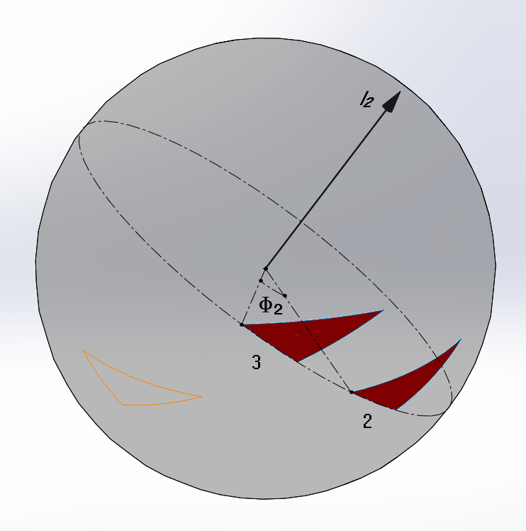
The view in Figure 16 is looking in the direction of the axis from the arrowhead side and is used to relate the screw displacements rotation angle $\Phi$, in this case clockwise between red-dashed perpendiculars at $\mathrm{1}$ and $\mathrm{3}$, to the angle $\theta$ between the half-turn perpendiculars $\mathrm{H_1}$ and $\mathrm{H_2}$ around the axis. Since $\Phi = α + β$ and $θ = \frac{α}{2} + \frac{\mathrm{β}}{2}$ then:
$$θ = \frac{\Phi}{2}\tag{23}$$
Figure 16
Combining Two Successive Screw Displacements
Figure 17 shows the idea of two successive screw displacements being replaced by a single screw displacement. The first displacement moves the object from positions $\mathrm{1}$ to $\mathrm{2}$ and the second from $\mathrm{2}$ to $\mathrm{3}$. These are replaced by one resultant screw displacement which moves the object from $\mathrm{1}$ to $\mathrm{3}$.

Figure 17
In $1882$, French mathematician Georges Halphen first proved this result and a proof using half-turns will be shown here. Also, vectors will later be used to derive formulas which only need the $\vec{l}$, $\Phi$, $\mathrm{S}$ and $\mathrm{d}$ parameters of two successive screw displacement to find the parameters of the resultant screw displacement. Fortunately, this vector approach is not the typical, more obscure way that you find in textbooks.
A key point in this proof is that a common perpendicular exists between skewed screw axes of the two successive displacements. This sets your first half-turn perpendicular and is for both the second half-turn off the first screw axis and for the first half-turn off the second screw axis. As is apparent in Figure 18, the positioning of the other two half-turn perpendiculars, the first off the first axis and the second off the second axis, will now depend on the objects extra half-turn displacement position $\mathrm{2'}$ around the common perpendicular. From Figure 18:
- The first half-turn off the first axis moves the triad from it's initial location $\mathrm{1}$ to $\mathrm{2'}$.
- A second half-turn around the common half-turn perpendicular moves it from $\mathrm{2'}$ to $\mathrm{2}$.
- A third half-turn again around the common perpendicular moves it from $\mathrm{2}$ back to $\mathrm{2'}$.
- Finally the last half-turn off the second axis moves it from $\mathrm{2'}$ to it's final location $\mathrm{3}$.

Figure 18
Note that these two half-turn perpendiculars like the screw axes are assumed skewed to each other but there are other cases which they are not and these will be looked at later. To find the resultant screw axis let's look at the half-turns. The first half-turn moves the triad from $\mathrm{1}$ to $\mathrm{2'}$, the last half-turn moves it from $\mathrm{2'}$ to $\mathrm{3}$. The two skewed perpendiculars of these half-turns will also have a common perpendicular between them and since perpendicular distances from it to similar points at $\mathrm{1}$ and $\mathrm{3}$ are equal then this perpendicular line is collinear with the resultant screw axis for the displacement from $\mathrm{1}$ to $\mathrm{3}$. The resulting structure of three screw axes and three common half-turn perpendiculars is referred to as the screw triangle. This is shown in a common more compact form with the tips and tails of the screw axes touching the half-turn perpendiculars which have been highlighted green in Figure 19 and thus have length $\mathrm{h}_i$. Also shown are the angles $\theta_{ij}$ between pairs of half-turn perpendiculars with the order of the subscripts being the same as the order of the half-turns.

Figure 19
Before proceeding to both the geometric and vector analysis of combining successive screw displacements, the independence of object orientation from it's slide (i.e. rectilinear translation) needs to be pointed out. It should be obvious that slides do not change object orientation but orientations can be changed by rotations around axes. So if you have two successive screw displacements and you are interested in just the objects change in orientation then the slide components can be ignored. One thing to remember is that rotations are generally non-commutative so order of rotation around axes matters to what will be the final orientation.
For the screw triangle in Figure 20, each screw $s_i$ is fully specified by it's unit normal $\vec{l_i}$, rotation angle $\Phi_i$, slide distance $\mathrm{d_i}$ and location $\mathrm{S_i}$. These parameters are written within a brace notation $\big\{\vec{l_i}, \Phi_i, \mathrm{d_i}, \mathrm{S_i}\big\}$. For our three screws in Figure 20 we have the following values measured off CAD software that modeled this screw triangle example:
$$\begin{align} s_1&: \big\{(0.000000, 1.000000, 0.000000), 75.406^\circ, 2.311715, (1.2065, 0, -0.397253)\big\}\\ s_2&: \big\{(0.248398, 0.775381, -0.580589), -34.916^\circ, 1.38437516, (1.98205, -0.0717971, 0.752112)\big\}\\ s_3&: \big\{(-0.374394, 0.903483, 0.208679), 52.464^\circ, 2.15106828, (-0.439634, 0.427021, -2.63756)\big\} \end{align}$$ with associated $Q$ values calculated as:$$\begin{align} Q_1 &= (0.000000, 0.772971, 0.000000) \\ Q_2 &= (-0.0781194, -0.243852, 0.182591) \\ Q_3 &= (-0.184485, 0.445196, 0.102828) \end{align}$$
Unit normal's of the screw triangle axes are all located at the origin with their tips on the surface of a unit radius sphere. Let normal's $\vec{l_1}$, $\vec{l_2}$ be for the two successive screw displacements $s_1$, $s_2$ and normal $\vec{l_3}$ for the resultant screw displacement $s_3$. Given all this we will start by showing that the product of two rotations is a rotation by looking at Donkin's theorem.

Figure 20
In Figure 21 a, b, the first and second screw rotations through angles $\Phi_1$ and $\Phi_2$ respectively are shown moving a shape on the surface of the unit sphere. A right-hand convention will be used for positive rotations and note that $\Phi_2$ will have a negative value by this convention. Also, the shape and it's initial position can be arbitrary but a spherical triangle of certain proportions with a certain placement was chosen. This triangle is first rotated from position $1$ to $2$ through angle $\Phi_1$ around $\vec{l_1}$ then from position $2$ to $3$ through angle $\Phi_2$ around $\vec{l_2}$. However, the triangle can also be rotated from $1$ to $3$ through angle $\Phi_3$ around $\vec{l_3}$ into congruence with the result of the two successive rotations around $\vec{l_1}$ and $\vec{l_2}$. Dorkin's theorem just picks the size, shape and initial placement of this triangle to make this congruence obvious and the geometric relationship between these three rotations evident.

a
b

c
Figure 21
To understand the choice of spherical triangle shape, it's size and initial placement in Dorkin's theorem consider Figure 22. The great circles are shown of the rotations around $\vec{l_1}$, $\vec{l_2}$, $\vec{l_3}$. A blue spherical triangle is formed by arcs of these three great circles with vertices labelled $\mathrm{A}$, $\mathrm{B}$ and $\mathrm{C}$ and three line segments are extended from the origin to these vertices for future reference. The red triangle is shown in it's three locations, the size of the arc edges of the red triangle are chosen to be equal with corresponding arc edges of the blue triangle so all triangles are of equal size and shape.
The red triangle is initially placed so that the arc edge which corresponds to the blue triangles arc edge on $\vec{l_1}$'s great circle, is also on $\vec{l_1}$'s great circle and just the ends of these two edges touch. When the red triangle is rotated around $\vec{l_1}$ by $\Phi_1$ to position $\mathrm{2}$, another one of it's edges is made to correspond to the blue triangles arc edge on $\vec{l_2}$'s great circle, this edge is also on $\vec{l_2}$'s great circle and just the ends of these two edges touch. Finally, the third edge of the red triangle at the initial position corresponds to the blue triangles arc edge on $\vec{l_3}$'s great circle, it also is on $\vec{l_3}$'s great circle and just the ends of these two edges touch.
 Figure 22
In Figures 21, the red triangle was shown rotating on the surface of the unit radius sphere around vectors $\vec{l_1}$, $\vec{l_2}$ and $\vec{l_3}$ and these figures could be used to show how a rotation $\vec{l_3}$ is equivalent to the two successive rotations $\vec{l_1}$ and $\vec{l_2}$.
However, with the help of Figure 22 you can also show this result another way because the displacement for each of the rotations around the normals $\vec{l_i}$ is equivalent to a pair of half-turns of the red triangle around two lines extending from $\mathrm{O}$. At position $1$, the top arc of the red triangle was chosen to have length equal to arc $\overparen{\mathrm{AB}}$ of the blue triangle. From position $1$, the red triangle is half-turned around line $\mathrm{OA}$ on the surface of the sphere which brings it's top arc into congruence with the blue triangles bottom arc. A second half-turn around line $\mathrm{OB}$ on the surface of the sphere then brings that same arc into congruence with the top arc of the red traingle at position $\mathrm{2}$. Since this top arc has equal length to arc $\overparen{\mathrm{AB}}$, rotation of the red-triangle around $\vec{l_1}$ must be twice the length of $\overparen{\mathrm{AB}}$ and because a unit radius circle has arc lengths equal to their associated angles in radians then $\overparen{\mathrm{AB}} = \frac{1}{2}\Phi_1$. Similarly, a second arc of the red triangle was chosen to be the one on the great circle of $\vec{l_2}$ when at position $2$ and have length equal to $\overparen{\mathrm{BC}}$. Half-turning the red triangle at $\mathrm{2}$ around $\mathrm{OB}$ and then $\mathrm{OC}$ brings this second arc into congruence with the corresponding edge of the red triangle positioned at $\mathrm{3}$. So $\overparen{\mathrm{BC}} = \frac{1}{2}\Phi_2$. Finally, the remaining arc of the red triangle was chosen to be the one on the great circle of $\vec{l_3}$ when at position $3$ and to have a length equal to $\overparen{\mathrm{AC}}$. Half-turning the red triangle at $\mathrm{1}$ around $\mathrm{OA}$ and $\mathrm{OC}$ brings this remaining arc into congruence with the corresponding edge of the red triangle positioned at $\mathrm{3}$. So $\overparen{\mathrm{AC}} = \frac{1}{2}\Phi_3$. Thus the size of the triangles arc edges are chosen based on their corresponding angles of rotation, $\Phi_1$, $\Phi_2$ and $\Phi_3$.
Note that the lines $\mathrm{OA}$, $\mathrm{OB}$ and $\mathrm{OC}$ in Figure 22 are parallel with the green half-turn lines of the screw-triangle in Figure 20. Each line $\mathrm{OA}$, $\mathrm{OB}$ and $\mathrm{OC}$ is a common normal to vector pairs $(\vec{l_1}, \vec{l_3})$, $(\vec{l_1}, \vec{l_2})$ and $(\vec{l_2},\vec{l_3})$ respectively. This is obvious from Figure 22 since $\mathrm{OA}$, $\mathrm{OB}$ and $\mathrm{OC}$ are collinear with the line of intersection between the two planes of rotation normal to each vector pair of $\vec{l}$'s. Now since the green half-turn lines are common normals between pairs of screw axes then it follows that they will be parallel with common normals between the associated pairs of $\vec{l}$'s of these axes. We have also previously shown that half-turns around $\mathrm{OA}$, $\mathrm{OB}$ and $\mathrm{OC}$ will properly orientate our object and thus they are analogous to the half-turns around the green lines of the screw triangle.
Furthermore, we can see from the structure of the blue triangle and the line segments extending from $\mathrm{O}$ to $\mathrm{A}$, $\mathrm{B}$ and $\mathrm{C}$ that rotating the vertex $\mathrm{A}$ by $\frac{\Phi_1}{2}$ around $\vec{l_1}$ is on the plane $\mathrm{OAB}$ normal to $\vec{l_1}$ and brings it to $\mathrm{B}$ and then rotating by $\frac{\Phi_2}{2}$ around $\vec{l_2}$ is on the plane $\mathrm{OBC}$ normal to $\vec{l_2}$ and brings it to $\mathrm{C}$. Alternatively, rotating $\mathrm{A}$ by $\frac{\Phi_3}{2}$ around $\vec{l_3}$ is on the plane $\mathrm{OAC}$ normal to $\vec{l_3}$ and brings it to $\mathrm{C}$. Letting $a$, $b$ and $c$ be the position vectors of $\mathrm{A}$, $\mathrm{B}$ and $\mathrm{C}$, and examining their vector relationships with $\vec{l_1}$, $\vec{l_2}$ and $\vec{l_3}$ in Figure 22, we can derive the formula for $\vec{Q_3} = \tan\Big(\frac{\Phi_3}{2}\Big)\vec{l_3}$ in terms of $\vec{Q_1} = \tan\Big(\frac{\Phi_1}{2}\Big)\vec{l_1}$ and $\vec{Q_2} = \tan\Big(\frac{\Phi_2}{2}\Big)\vec{l_2}$.
Figure 23 is a version of Figure 22, simplified to look at the first rotation of vertex $\mathrm{A}$ to $\mathrm{B}$. Let point $\mathrm{M}$ be colinear with $\mathrm{OB}$, $\mathrm{M}$ is off the surface of the sphere and $\mathrm{M}$ is intersected by the perpendicular to vector $\vec{a}$ that extends from point $\mathrm{A}$. Letting $\vec{m}$ be the position vector of $\mathrm{M}$ we derive the formula for point $\mathrm{B}$.

Figure 23
Since $\tan\Big(\frac{\Phi_1}{2}\Big) = \left|\left|\vec{m} - \vec{a}\right|\right|\big/\left|\left|\vec{a}\right|\right|$ then:
$$\vec{m} - \vec{a} = \tan\Big(\frac{\Phi_1}{2}\Big)\vec{l_1} \times \vec{a}\tag{25}$$ $$\vec{m} = \vec{a} + \vec{Q_1} \times \vec{a}\tag{26}$$The unit vector for $\vec{m}$ is the position vector $\vec{b}$ and therefore:
$$\begin{align} \vec{b} &= \frac{\vec{m}}{\left|\left|\vec{m}\right|\right|}\\ \\ &= \frac{\vec{a} + \vec{Q_1} \times \vec{a}}{\left|\left|\vec{a} + \vec{Q_1} \times \vec{a}\right|\right|}\tag{27} \end{align}$$Similarily, going from $\mathrm{B}$ to $\mathrm{C}$:
$$\vec{c} = \frac{\vec{b} + \vec{Q_2} \times \vec{b}}{\left|\left|\vec{b} + \vec{Q_2} \times \vec{b}\right|\right|}\tag{28}$$Finally, from $\mathrm{A}$ to $\mathrm{C}$:
$$\vec{c} = \frac{\vec{a} + \vec{Q_3} \times \vec{a}}{\left|\left|\vec{a} + \vec{Q_3} \times \vec{a}\right|\right|}\tag{29}$$Inserting equation $(27)$ into $(28)$ gives:
$$\vec{c} = \frac{\vec{a} + \vec{Q_1} \times \vec{a} + \vec{Q_2} \times \vec{a} + \vec{Q_2} \times (\vec{Q_1} \times \vec{a})}{\left|\left|\vec{a} + \vec{Q_1} \times \vec{a} + \vec{Q_2} \times \vec{a} + \vec{Q_2} \times (\vec{Q_1} \times \vec{a})\right|\right|}\tag{30}$$Equating the right-hand sides of $(29)$ and $(30)$:
$$\frac{\vec{a} + \vec{Q_3} \times \vec{a}}{\left|\left|\vec{a} + \vec{Q_3} \times \vec{a}\right|\right|} = \frac{\vec{a} + \vec{Q_1} \times \vec{a} + \vec{Q_2} \times \vec{a} + \vec{Q_2} \times (\vec{Q_1} \times \vec{a})}{\left|\left|\vec{a} + \vec{Q_1} \times \vec{a} + \vec{Q_2} \times \vec{a} + \vec{Q_2} \times (\vec{Q_1} \times \vec{a})\right|\right|}\tag{31}$$The numerator and denominator of $(31)$'s left-side can be multiplied by the same constant $\mathrm{k}$ without affecting the ratio on that side:
$$\bigg(\frac{\mathrm{k}}{\mathrm{k}}\bigg)\Bigg(\frac{\vec{a} + \vec{Q_3} \times \vec{a}}{\left|\left|\vec{a} + \vec{Q_3} \times \vec{a}\right|\right|}\Bigg) = \frac{\vec{a} + \vec{Q_1} \times \vec{a} + \vec{Q_2} \times \vec{a} + \vec{Q_2} \times (\vec{Q_1} \times \vec{a})}{\left|\left|\vec{a} + \vec{Q_1} \times \vec{a} + \vec{Q_2} \times \vec{a} + \vec{Q_2} \times (\vec{Q_1} \times \vec{a})\right|\right|}\tag{32}$$Constant $\mathrm{k}$ can then be chosen so both numerators are equal:
$$\mathrm{k}(\vec{a} + \vec{Q_3} \times \vec{a}) = \vec{a} + \vec{Q_1} \times \vec{a} + \vec{Q_2} \times \vec{a} + \vec{Q_2} \times (\vec{Q_1} \times \vec{a})\tag{33}$$Using the vector triple product of $\vec{Q_2} \times (\vec{Q_1} \times \vec{a})$ which is $(\vec{Q_2} \cdot \vec{a})\vec{Q_1} - (\vec{Q_2} \cdot \vec{Q_1})\vec{a}$ gives:
$$\mathrm{k}(\vec{a} + \vec{Q_3} \times \vec{a}) = \vec{a} + \vec{Q_1} \times \vec{a} + \vec{Q_2} \times \vec{a} + (\vec{Q_2} \cdot \vec{a})\vec{Q_1} - (\vec{Q_2} \cdot \vec{Q_1})\vec{a}\tag{34}$$Rearranging and combining terms:
$$\mathrm{k}(\vec{Q_3} \times \vec{a}) + ((\vec{Q_2} \cdot \vec{Q_1}) - 1 + \mathrm{k})\vec{a} = (\vec{Q_1} \times \vec{a}) + (\vec{Q_2} \times \vec{a}) + (\vec{Q_2} \cdot \vec{a})\vec{Q_1}\tag{35}$$Using the vector triple product expansion $-(\vec{a} \cdot \vec{Q_1})\vec{Q_2} + (\vec{a} \cdot \vec{Q_2})\vec{Q_1} = (\vec{Q_2} \times \vec{Q_1}) \times \vec{a}$ and taking into account that $\vec{a}$ is perpendicular to $\vec{Q_1}$ we then omit the term $(\vec{a} \cdot \vec{Q_1})\vec{Q_2}$. This gives $(\vec{a} \cdot \vec{Q_2})\vec{Q_1} = (\vec{Q_2} \times \vec{Q_1}) \times \vec{a}$ which is substituted into $(35)$:
$$\mathrm{k}(\vec{Q_3} \times \vec{a}) + ((\vec{Q_2} \cdot \vec{Q_1}) - 1 + \mathrm{k})\vec{a} = (\vec{Q_1} \times \vec{a}) + (\vec{Q_2} \times \vec{a}) + (\vec{Q_2} \times \vec{Q_1}) \times \vec{a}\tag{36}$$Except for one summand in equation $(36)$, all other summands are perpendicular to $\vec{a}$ because they are each cross products of $\vec{a}$ with another vector. The exception is $((\vec{Q_2} \cdot \vec{Q_1}) - 1 + \mathrm{k})\vec{a}$ which just scales $\vec{a}$ and thus is obviously parallel to $\vec{a}$. Since the right-hand side of $(36)$ result in a vector perpenducular to $\vec{a}$ then $(36)$ can only be true if the left-hand side does as well. So the exception summand has to be zero, that is, $\vec{Q_2} \cdot \vec{Q_1} - 1 + \mathrm{k} = 0$. Inserting $\mathrm{k} = 1 - \vec{Q_2} \cdot \vec{Q_1}$ into equation $(36)$ we get:
$$(1 - \vec{Q_2} \cdot \vec{Q_1})(\vec{Q_3} \times \vec{a}) = (\vec{Q_1} \times \vec{a}) + (\vec{Q_2} \times \vec{a}) + (\vec{Q_2} \times \vec{Q_1}) \times \vec{a}\tag{37}$$Hence
$$\vec{Q_3} \times \vec{a} = \frac{\vec{Q_1} + \vec{Q_2} + \vec{Q_2} \times \vec{Q_1}}{1 - \vec{Q_2} \cdot \vec{Q_1}} \times \vec{a}\tag{38}$$Finally
$$\vec{Q_3} = \frac{\vec{Q_1} + \vec{Q_2} + \vec{Q_2} \times \vec{Q_1}}{1 - \vec{Q_2} \cdot \vec{Q_1}}\tag{39}$$For our example, the calculated value of $\vec{Q_3}$ from $(39)$ is:
$$\vec{Q_3} = \frac{(-0.219257, 0.529119, 0.122207)}{1.18849} = (-0.184484, 0.445203, 0.102825)$$Next, we will find angle $\Phi_3$ from the spherical law of cosines for triangle $\mathrm{ABC}$.
$$\cos \Big(\frac{\Phi_3}{2}\Big) = \cos \Big(\frac{\Phi_1}{2}\Big)\cos \Big(\frac{\Phi_2}{2}\Big) - \cos \Big(\alpha\Big)\sin \Big(\frac{\Phi_1}{2}\Big)\sin \Big(\frac{\Phi_2}{2}\Big)\tag{40}$$ where $\cos(\alpha) = \left|\left|\vec{l_1} \cdot \vec{l_2}\right|\right|$. For our values, $\cos(\alpha) = 0.775381$ and$$\begin{align} \cos \Big(\frac{\Phi_3}{2}\Big) &= (0.791192)(0.953937) - (0.775381)(0.611568)(-0.300007) \\ &= 0.897010 \\ \\ \Phi_3 &= 2 \cos^{-1}(0.897010) = 52.46^\circ \end{align}$$ Hence
$$\vec{l_3} = \frac{(-0.184484, 0.445203, 0.102825)}{\tan(26.23^\circ)} = (-0.374426, 0.903577, 0.208692)$$
Finally, given $\vec{l_3}$ and $\Phi_3$, we will find the slide distance $\mathrm{d_3}$ and then the location of $s_3$. It was mentioned before that the intersection point of a line from the origin $\mathrm{O}$ that is perpendicular to the screw axis is used as it's location point. In Figure 24, three black dashed lines are these perpendiculars, they intersect screws $s_1$, $s_2$, $s_3$ at points $\mathrm{S_1}$, $\mathrm{S_2}$, $\mathrm{S_3}$.

Figure 24
If $s_1$ was applied on a point to place it at a final position $\mathrm{S_2}$ then we can find it's initial position $\mathrm{S^{'}_{2}}$ by using equation $(21)$, but modifying it for a right-hand positive rotation convention which changes the order of the vector pairs in the cross-product term. Letting $\mathrm{X} = \mathrm{S_2} - \mathrm{S_1} - (\mathrm{d_1})\vec{l_1}$ gives:
$$\mathrm{S^{'}_{2}} = \mathrm{X}\cos(\Phi_1) + \big(\mathrm{X}\sin(\Phi_1)\big) \times \vec{l_1} + \big(\mathrm{X}\cdot \vec{l_1}\big) \vec{l_1} \big( 1 - \cos(\Phi_1)\big) + \mathrm{S_1}\tag{41}$$ $$\begin{align} \mathrm{X} &= (0.77555, -2.38351, 1.14937) \\ \\ \mathrm{S^{'}_{2}} &= (0.195414, -0.600568, 0.289604) \\ &+ (-1.11229, 0, 0.750527) \\ &+ (0, -1.78287, 0) \\ &+ (1.2065, 0, -0.397253) \\ \\ &= (0.289624, -2.38344, 0.642878) \end{align}$$which closely agrees with the measured value $(0.289635, -2.38351, 0.642876)$.
When $s_2$ is applied on point $\mathrm{S_2}$ then it will only slide that point a distance $\mathrm{d_2}$ along $s_2$ to it's final position $\mathrm{S^{"}_{2}}$ which is found with:
$$\begin{align} \mathrm{S^{"}_{2}} &= \mathrm{S_2} + (\mathrm{d_2})\vec{l_2}\tag{42} \\ \\ &= (1.98205, -0.071798, 0.752112) + (1.38438)(0.248398, 0.775381, -0.580589) \\ &= (2.32593, 1.00162, -0.051644) \end{align}$$which closely agrees with the measured value $(2.32593, 1.00162, -0.0516412)$.
The slide distance $\mathrm{d_3}$ is then:
$$\begin{align} \mathrm{d_3} &= (\mathrm{S^{"}_{2}} - \mathrm{S^{'}_{2}}) \cdot \vec{l_3}\tag{43} \\ \\ &= (2.03631, 3.38506, -0.694522) \cdot (-0.374394, 0.903483, 0.208679)\\ &= 2.15103 \end{align}$$Finally, to find $\mathrm{S_3}$ with points $\mathrm{S^{'}_{2}}$ and $\mathrm{S^{"}_{2}}$, use the following version of equation $(14)$ which is again modified for a right-hand positive rotation convention that changes the order of the vector pairs in the cross-product terms:
$$\begin{align} \mathrm{S_3} &= \frac{\vec{Q_3} \times \big(\mathrm{S^{"}_{2}} - \mathrm{S^{'}_{2}} - \vec{Q_3} \times (\mathrm{S^{"}_{2}} + \mathrm{S^{'}_{2}}) \big)}{2\vec{Q_3} \cdot \vec{Q_3}}\tag{44} \\ \\ &= \frac{(-0.213503, 0.207373, -1.28088)}{0.485616}\\ \\ &= (-0.439654, 0.427031, -2.63764) \end{align}$$Now let's look at some edge cases with the screw-triangle. Note that the following figures use a left-hand screw because this gives a better view of the spirals.
First as shown in Figure 25, if either of the screws $s_1$, $s_2$ have no rotation and only a slide occurs like with screw $s_1$ then this screw will have both it's half-turn lines parallel and the resultant screw $s_3$ will have $\vec{l_3}$ parallel with the other screw $s_2$. So $\vec{l_3}$ and $\vec{l_2}$ are parallel, $\Phi_3 = \Phi_2$ and equations $(42)$, $(43)$ and $(44)$ are used to find $\mathrm{d_3}$ and $\mathrm{S_3}$.

Figure 25
Second, what if axes $s_1$ and $s_2$ are not skewed but parallel like in Figure 26? No unique common perpendicular exists between them, the rotational portions of their displacements will be on parrallel planes so the resultant screw $s_3$ will be parallel to $s_1$ and $s_2$. This means that $\vec{l_1}$, $\vec{l_2}$ and $\vec{l_3}$ are parallel, the angle $\left|\left|\Phi_3\right|\right| = \left|\left|\Phi_1 \pm \Phi_2\right|\right|$ and equations $(42)$, $(43)$ and $(44)$ are used to find $\mathrm{d_3}$ and $\mathrm{S_3}$.

Figure 26

